r = (1/a)cosh(az).
In cat.fe, both the upper and lower rings are given as one-parameter
boundary wires. The separation and radius are parameters, so
you can change them during a run with assignment statements or the
A command.
The initial radius given is the minimum for which a catenoid can exist
for the given separation of the rings. To get a stable catenoid, you
will have to increase this value. However, if you do run with the
original value, you can watch the neck pinch out.
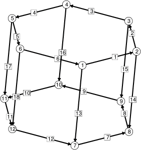
The initial surface
consists of six rectangles forming a cylinder between the two circles.
The vertices on the boundaries are fixed, elsewise they would slide
along the boundary to short-cut the curvature; two diameters is shorter
than one circumference. The boundary edges are fixed so that vertices arising
from subdividing the edges are likewise fixed.
 |
The initial catenoid skeleton, with vertices and edges numbered. |
// cat.fe
// Evolver data for catenoid.

PARAMETER  RMAX = 1.5088795   // minimum radius for height
PARAMETER  ZMAX = 1.0

boundary 1 parameters 1     //  upper ring
x1:  RMAX * cos(p1)
x2:  RMAX * sin(p1)
x3:  ZMAX

boundary 2 parameters 1    //   lower ring
x1:  RMAX * cos(p1)
x2:  RMAX * sin(p1)
x3:  -ZMAX

vertices   // given in terms of boundary parameter
1    0.00  boundary 1   fixed
2    pi/3  boundary 1   fixed
3  2*pi/3  boundary 1   fixed
4    pi    boundary 1   fixed
5  4*pi/3  boundary 1   fixed
6  5*pi/3  boundary 1   fixed
7    0.00  boundary 2   fixed
8    pi/3  boundary 2   fixed
9  2*pi/3  boundary 2   fixed
10   pi    boundary 2   fixed
11 4*pi/3  boundary 2   fixed
12 5*pi/3  boundary 2   fixed

edges
1    1  2  boundary 1   fixed
2    2  3  boundary 1   fixed
3    3  4  boundary 1   fixed
4    4  5  boundary 1   fixed
5    5  6  boundary 1   fixed
6    6  1  boundary 1   fixed
7    7  8  boundary 2   fixed
8    8  9  boundary 2   fixed
9    9  10 boundary 2   fixed
10   10 11 boundary 2   fixed
11   11 12 boundary 2   fixed
12   12 7  boundary 2   fixed
13   1  7
14   2  8
15   3  9
16   4  10
17   5  11
18   6  12

faces
1   1 14 -7 -13
2   2 15 -8 -14
3   3 16 -9 -15
4   4 17 -10 -16
5   5 18 -11 -17
6   6 13 -12 -18
The parameter in a boundary definition is always
p1 (and p2
in a two-parameter boundary). The Evolver can handle periodic parameterizations,
as is done in this example.
Try this sequence of
commands (displaying at your convenience):
    r       (refine to get a crude, but workable, triangulation)
    u       (equiangulation makes much better triangulation)
    g 120   (takes this many iterations for neck to collapse)
    t 0.05  (collapse neck to single vertex by eliminating all
                      edges shorter than 0.05)
    o       (split neck vertex to separate top and bottom surfaces)
    g       (spikes collapse)
The catenoid shows some of the subtleties of evolution. Suppose the
initial radius is set to RMAX = 1.0 and the initial height to
ZMAX = 0.55 (these are pre-set in catman.fe).
Fifty iterations with optimizing scale factor result in an area of 6.458483.
At this point, each iteration is reducing the area by only .0000001,
the triangles are all nearly equilateral, everything
looks nice, and the innocent user might conclude the surface is very
near its minimum. But this is really a saddle point of energy.
Further iteration shows that the area change per iteration bottoms out
about iteration 70, and by iteration 300 the area is down to 6.4336.
The triangulation really wants to twist around so that there are edges
following the lines of curvature, which are vertical meridians and
horizontal circles. Hence the optimum triangulation appears to be
rectangles with diagonals.
The evolution can be speeded up by turning on the
conjugate gradient
method with the
U
command.
With catman.fe, try the script "r; u; U; g 70".
For conjugate gradient cognoscenti,
the saddle point demonstrates the difference between the Fletcher-Reeves
and Polak-Ribiere versions of conjugate gradient. The saddle point
seems to confuse the Fletcher-Reeves version (which used to be the default).
However, the Polak-Ribiere version (the current default) has little problem.
The
U
command toggles conjugate gradient on and off, and
ribiere
toggles the Polak-Ribiere version.
With Fletcher-Reeves conjugate gradient in effect, the
saddle point is reached at iteration 17 and area starts decreasing again
until iteration 30, when it reaches 6.4486. But then iteration stalls
out, and the conjugate gradient mode has to be turned off and on to
erase the history vector. Once restarted, another 20 iterations will
get the area down to 6.4334.
In Polak-Ribiere mode, no restart is necessary.
Exercise for the reader: Get the Surface Evolver to display an unstable
catenoid by declaring the catenoid facets to be the boundary of a body,
and adjusting the body volume with the
b
command to get zero pressure.
See the sample datafile catbody.fe.