The effect of the rotation is incorporated in the energy through an integral using the Divergence Theorem:
        ///
  E = - ||| (1/2) p r^2 w^2 dV
	///B

        //
    = - ||       (1/2) p w^2 (x^2+y^2) z k·dA
        //bdry B
where B is the region of the liquid, r is radius from the axis,
p is the fluid density and w is the angular velocity.
Note the energy is negative, because spin makes the liquid want to move
outward. This has to be countered by surface tension forces holding
the liquid on the rod. If p is negative, then one has a toroidal
bubble in a rotating liquid, and high spin stabilizes the torus.
The spin energy is put in the datafile using the named quantity syntax
(see below).
"centrip" is a user-chosen name for the quantity, "energy"
declares that this quantity is part of the total energy,
"global_method"
says that the following method is to be applied to the whole surface,
"facet_vector_integral" is the pre-defined name of the method
that integrates vector fields over facets, and "vector_integrand"
introduces the components of the vectorfield.
The rod surface is defined to be constraint 1 with equation x^2 + y^2 = R^2, where R is the radius of the rod. The contact energy of the liquid with the rod is taken care of with an edge integral over the edges where the liquid surface meets the rod:
      //                          /                  /
  E = || -T cos(a) dA = -T cos(a) |  z ds = T cos(a) | (z/R)(yi - xj)·ds
      //S                         /bdry S            / bdry S
Here S is the rod surface not included as facets in bdry B,
T is the surface tension of the free surface, and a is the
internal contact angle. A more intuitive way to arrive at this integral
is to think in cylindrical coordinates and
imagine the replaced surface of the rod between the contact line and
z = 0 to be divided into thin vertical strips of height z and width R dtheta.
The energy of a strip is -T cos(a) z R dtheta. Converting back
to Cartesian coordinates, dtheta = (x dy - y dx)/(x^2 + y^2), so
                 //                                   //
  E =  -T cos(a) || z R (x dy - y dx)/R^2 = -T cos(a) || (z/R)(x dy - y dx)
                 //                                   //
Constraint 2 is a horizontal symmetry plane. By assuming symmetry, we only have to do half the work.
Constraint 3 is a one-sided constraint that keeps the liquid outside the rod. Merely having boundary edges on the rod with constraint 1 is not enough in case the contact angle is near 180 degrees and the liquid volume is large. Constraint 3 may be put on any vertices, edges, or faces likely to try to invade the rod. However, it should be noted that if you put constraint 3 on only some vertices and edges, equiangulation will be prevented between facets having different constraints.
Constraint 4 is a device to keep the vertices on the rod surface evenly
spaced. Edges on curved constraints often tend to become very uneven,
since long edges short-cutting the curve can save energy. Hence the
need for a way to keep the vertices evenly spread circumferentially, but
free to move vertically. One way to do that is with another constraint
with level sets being vertical planes through the z axis
at evenly spaced angles. Constraint 4 uses the real modulus
function with arctangent to create a periodic constraint. Each refinement,
the parameters need to be halved to cut the period in half. This is done
by redefining the "r" refinement command at the end of the datafile.
Note that autorecalc is temporarily turned off to prevent projecting
vertices to the constraint when it is in an invalid state. Also note the
pi/6 offset to avoid the discontinuity in the modulus function.
pi/6 was cleverly chosen so that all refinements would also avoid
the discontinuity.
One way of detecting stability is to perturb the torus and seeing if it evolves back to equilibrium. The datafile defines a command
perturb := set vertex y y+.01 where not on_constraint 1
This sets the y coordinate of each vertex to y+.01.
This command is defined in the "read" section
at the end of the datafile, where you can put whatever commands you
want to execute immediately after the datafile is loaded.
To detect small perturbations, and get numerical values for the size
of perturbations, the y moment of the liquid is calculated in the
named quantity "ymoment". It is not part of the energy, as
indicated by the info_only keyword. You can see the value
with the `v' command.
A better way to check stability is to examine the eigenvalues of
the Hessian matrix. First, evolve normally to reasonably near
an equilibrium. Then use the hessian
command several times to converge exactly to the equilibrium. Then
use the command "ritz(0,5)"
to display the 5 eigenvalues of
the Hessian nearest 0. By gradually raising the spin and tracking
the lowest eigenvalue, one can detect the onset of instability, where
the lowest eigenvalue becomes 0. Note that the datafile toggles on
hessian_normal so that the
Hessian only considers perturbations normal to the surface.
 |
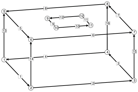
The initial ringblob skeleton, with vertices and edges numbered. Taking advantage of symmetry, just the top half is represented. |
// ringblob.fe

// Toroidal liquid ring on a rotating rod in weightlessness.
// Half of full torus
// Using second periodic constraint surface intersecting rod to
// confine vertices on rod to vertical motion.

// Important note to user: Use only the 'rr' command defined at
// the end of this file to do refinement.  This is due to the
// nature of constraint 4 below.

// This permits drawing both halves of the ring
view_transforms 1
1 0 0 0
0 1 0 0
0 0 -1 0
0 0 0 1

// Basic parameters.  These may be adjusted at runtime with the
// 'A' command.  Only spin is being adjusted in these experiments.
parameter rodr = 1  // rod radius
parameter spin = 0.0 // angular velocity
parameter angle = 30 // internal contact angle with rod
parameter tens = 1   // surface tension of free surface
#define rode (-tens*cos(angle*pi/180))  // liquid-rod contact energy
parameter dens = 1  // density of liquid, negative for bubble

// spin centripetal energy
quantity centrip energy global_method facet_vector_integral
vector_integrand:
q1: 0
q2: 0
q3: -0.5*dens*spin*spin*(x^2+y^2)*z

// y moment, for detecting instability
quantity ymoment info_only global_method facet_vector_integral
vector_integrand:
q1: 0
q2: 0
q3: y*z

// Constraint for vertices and edges confined to rod surface,
// with integral for blob area on rod
constraint 1
formula: x^2 + y^2 = rodr^2
energy:
e1: -rode*z*y/rodr
e2: rode*z*x/rodr
e3: 0

// Horizontal symmetry plane
constraint 2
formula: z = 0

// Rod surface as one-sided constraint, to keep stuff from caving in
// Can be added to vertices, edges, facets that try to cave in
constraint 3 nonnegative
formula: x^2 + y^2 = rodr^2

// Constraint to force vertices on rod to move only vertically.
// Expressed in periodic form, so one constraint fits arbitrarily
// many vertices. Note offset to pi/6 to avoid difficulties with
// modulus discontinuity at 0.
parameter pp = pi/2    /* to be halved each refinement */
parameter qq = pi/6    /* to be halved each refinement */
constraint 4
formula:  (atan2(y,x)+pi/6) % pp = qq

//initial dimensions
#define ht 2
#define wd 3

vertices
1  0   -wd 0  constraints 2    // equatorial vertices
2  wd    0 0  constraints 2
3  0    wd 0  constraints 2
4  -wd   0 0  constraint 2
5  0   -wd ht                 // upper outer corners
6  wd    0 ht
7  0    wd ht
8  -wd   0 ht
9  0 -rodr ht constraints 1,4   // vertices on rod
10 rodr  0 ht constraints 1,4
11 0  rodr ht constraints 1,4
12 -rodr  0 ht constraints 1,4

edges
1   1 2 constraint 2  // equatorial edges
2   2 3 constraint 2
3   3 4 constraint 2
4   4 1 constraint 2
5   5 6               // upper outer edges
6   6 7
7   7 8
8   8 5
9   9  10 constraint 1,4   // edges on rod
10  10 11 constraint 1,4
11  11 12 constraint 1,4
12  12  9 constraint 1,4
13   1  5        // vertical outer edges
14   2  6
15   3  7
16   4  8
17   5  9        // cutting up top face
18   6 10
19   7 11
20   8 12

faces  /* given by oriented edge loop */
1   1 14 -5 -13 tension tens // side faces
2   2 15 -6 -14 tension tens  // Remember you can't change facet tension
3   3 16 -7 -15 tension tens  // dynamically just by changing tens; you have
4   4 13 -8 -16 tension tens  // to do "tens := 2; set facet tension tens"
5   5 18 -9 -17 tension tens  // top faces
6   6 19 -10 -18 tension tens
7   7 20 -11 -19 tension tens
8   8 17 -12 -20 tension tens

bodies  /* one body, defined by its oriented faces */
1   1 2 3 4 5 6 7 8  volume 25.28

read  // some initializations
transforms off     // just show fundamental region to start with

// special refinement command redefinition
r :::= { autorecalc off;  pp := pp/2; qq := qq % pp; 'r'; autorecalc on; }

// a slight perturbation, to check stability
perturb := set vertex y y+.01 where not on_constraint 1

hessian_normal // to make Hessian well-behaved
linear_metric  // to normalize eigenvalues