Surface Evolver Workshop Day 6

Trinity College Surface Evolver Workshop

Surface Evolver Workshop Day 6

Higher order elements

You need an awful lot of flat triangles to accurately approximate a curved surface. In general, each refinement will reduce the error in the area by a factor of 4, at the expense of a 4-fold increase in the number of vertices. Not very efficient. A better approximation can be done by using curved elements instead of flat elements. With triangular facets, the obvious scheme is to have each facet be the image of a triangular domain { (u,v) | 0 <= u <= 1 and 0 <= v < u } under polynomial maps x(u,v), y(u,v), and z(u,v). An order N polynomial in two variables needs (N+1)(N+2)/2 coefficients, and a nice geometric way to supply them is to prescribe (N+1)(N+2)/2 "control points" in (x,y,z) that the image must pass through. In the world of finite elements, this scheme is known as "Lagrange elements". There are other ways of specifying the coefficients (Bezier splines, Hermite splines, etc.) but they all wind up specifying the same class of geometric surfaces.

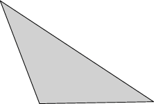
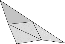
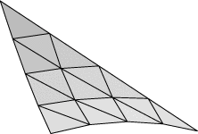
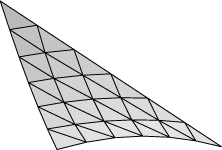
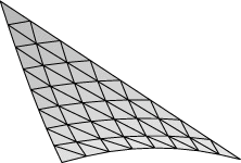
Evolver implements Lagrange elements up through order 8. Here are pictured a single facet in various orders, meshed with their control points:


Order 1 (linear)	Order 2 (quadratic)	Order 4

Order 6	Order 8

The facets are actually much smoother than the pictures show; they are just drawn with flat sub-triangles instead of the real curved surfaces.

Higher-order elements can more accurately represent a surface, but they have the disadvantage of taking more time to compute. Below is a table showing the tradeoff between accuracy and speed for the file cube.fe:

Accuracy and hessian time for cube.fe
	Lagrange order
Refinement	1	2	4	6	8
0	0.276517266 < 0.01 sec	0.004335146 0.06 sec	2.37245E-06 0.23 sec	4.10881E-08 0.80 sec	3.95497E-11 3.916 sec
1	0.068570688 < 0.01 sec	6.91458E-05 0.06 sec	2.32691E-09 0.46 sec	2.60947E-12 3.07 sec	9E-15 16.04 sec
2	0.017587463 0.03 sec	1.05169E-06 0.23 sec	2.35012E-12 1.92 sec	1.6E-16 12.61 sec	1e-18 63.40 sec
3	0.004459441 0.15 sec	1.61997E-08 1.03 sec	9E-15 8.50 sec	1E-18 52.90 sec
4	0.001120878 0.65 sec	2.5231E-10 5.30 sec	2E-18 42.58 sec	1E-18 234.16 sec
5	0.000280722 4.98 sec	3.94973E-12 31.53 sec

Note how fast the error decreases with refinement for each order.

Order	Improvement factor
1	4
2	64
4	1024
6	16384
8	lots

Really fantastic. Unfortunately, most surfaces aren't as smooth as a sphere. For quad.fe the results look like this:

Accuracy and hessian time for quad.fe
	Lagrange order
Refinement	1	2	4	6	8
0	0.087900176 < 0.01 sec	0.000109299 < 0.01 sec	7.56228E-07 0.01 sec	2.88111E-08 0.08 sec	2.55843E-09 0.23 sec
1	0.021300761 < 0.01 sec	1.98468E-05 0.01 sec	3.95907E-08 0.02 sec	1.36209E-09 0.16 sec	1.2269E-10 0.81 sec
2	0.005296499 < 0.01 sec	1.81652E-06 0.01 sec	1.97628E-09 0.10 sec	6.61498E-11 0.67 sec	6.00E-12 3.44 sec
3	0.00132285 0.01 sec	1.40166E-07 0.05 sec	9.65104E-11 0.44 sec	3.240E-12 2.92 sec	2.89E-13 14.33 sec
4	0.000330656 0.03 sec	9.99313E-09 0.24 sec	4.72E-12 2.02 sec	1.5E-13 12.26 sec	1.0E-14 59.02 sec
5	8.26616E-05 0.12 sec	6.8302E-10 1.16 sec	2.2E-13 9.06 sec	1E-15 52.01 sec
6	2.06653E-05 0.62 sec	4.54996E-11 5.88 sec	1E-15 43.24 sec

The improvement factor peaks out at about 20. Still a lot better than the linear model. Looking at the times shows there is no clearly fastest way to get a given accuracy. Order 8 tends to be slower than order 6 for the same accuracy. I tend to use order 6 when I want high accuracy, but the best choice may vary among surfaces.

As practice with higher-order elements, run conserved.fe and set the volume so the area of the ideal sphere is exactly 1:

 body[1].target := 4/3*pi*(1/4/pi)^(3/2)

I suggest conserved.fe rather than cube.fe since the zero eigenvalues of translational degrees of freedom give much more trouble for the hessian in higher orders. You can set the order of the elements with the 'M' command followed by the order, as in "M 2". "linear" is a synonym for "M 1", "quadratic" is a synonym for "M 2", and "lagrange n" is a synonym for "M n". Try this evolution:

 body[1].target := 4/3*pi*(1/4/pi)^(3/2)
  g 5;
  hessian; 
  hessian; 
  M 2;
  g 5;
  hessian;
  hessian; 
  M 4;
  g 5;
  hessian;
  hessian; 
  M 6;
  g 5;
  hessian;
  hessian; 
  M 8;
  g 5;
  hessian;
  hessian;

Note: Internally, the lagrange code was added after the linear and quadratic code, so "linear" is not technically the same as "lagrange 1" (but the effects are the same), and "quadratic" is not exactly "lagrange 2". More mesh operations like refine, delete, equiangulate, etc are defined for linear and quadratic mode than for lagrange mode, so there is no real reason to use "lagrange 1" or "lagrange 2". In general, you want to do all your refining, mesh grooming, and coarse evolution in linear mode, and only switch to higher order modes to get the final precision.

The datafile can be set up directly in quadratic mode by including the "quadratic" keyword in the top section of the datafile, defining a midpoint vertex for each edge as normally done for vertices, and then listing the midpoint vertex as the THIRD vertex on the edge definition line. Nothing is different for facets. Higher order Lagrange elements can also be set up, but I have never done this by hand; but dump files use this feature.

Ultra-high precision

Most computers implement 64-bit floating point numbers as standard, which gives 14 to 15 digits of precision. Some machines can do more in hardware (Intel x86 has an 80-bit floating point type with 18 to 19 digits of precision) or software (128 bit floating point on many unix systems for 30 digits of precision). These extended precision floating point types are of type "long double" in C. Evolver is written so the type of all internal floating point numbers can be set with a compile-time option, -DLONGDOUBLE. This high-precision version is available to you in my bin directory as evolverLD. If you think numerical precision is affecting your results, or you just want to see how accurate higher order Lagrange elements can be, run this version.

Run evolverLD on conserved.fe and compare the results of the above evolution to see what effect the increased accuracy has.

Note: You will see that the output of the 'g' command does not print area any more. With the extended precision, there just isn't room on an 80-column line for both area and energy.

Circular arcs in the string model

Two-dimensional foams governed purely by surface tension are made up of circular arcs. The Evolver now has a mode that represents edges in the string model as exact circular arcs. Defining a circular arc geometrically in terms of vertices requires two endpoints and a midpoint, which is the same information that quadratic mode uses, so circular arc mode is implemented as a submode of quadratic mode. The alteration is to use special circular arc length and area calculations. These are implemented as named methods, circular_arc_length and circular_arc_area. These can be used as stand-alone methods, but I wanted to actually replace the default length and area calculations, so the datafile syntax I chose is to put these lines in the top of the datafile:

area_method_name "circular_arc_area"
length_method_name "circular_arc_length"

This is implementing a general method for substituting named methods for the default area and length, but so far circular_arc is the only real use I've had for it.

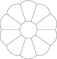
To see circular arc mode in action, run flowerarc.fe. It starts in ordinary linear mode. To turn on circular arc mode, do "M 2" or "quadratic". Then evolve "g 15". You have complete convergence, with no need to refine or use higher order elements.

To see the accuracy of circular arc mode, run circle_arc.fe. This has a circle of area pi made out of four edges. Evolve with "M 2; g 5;" and compare the energy to the ideal 2*pi (which you can find with "print 2*pi").

In circular arc mode, edges are drawn as 16 short straight lines, so they look pretty circular. However, in PostScript output, the edges are drawn as exact PostScript arcs.

Circular arc mode is compatible with torus mode. Clipping works correctly (although clipping circular arcs is a much bigger pain than clipping straight edges).

Writing commands and scripts

The Evolver commands used so far in this workshop have been pretty short and simple. But the time comes when you want to write more complicated commands. Some typical uses of user-defined commands:

Do some standard initial operations on the surface when its loaded, refining certain edges, etc.
Recording evolutions that work well for a datafile. It takes some effort to work out a good and efficient evolution, and you should put it in a command when you find one. I emphasize "efficient"; I see too many evolution scripts that do hundreds or thousands when ten would do. Use conjugate gradient as soon as possible. Use hessian (rather, hessian_seek) as soon as possible. Don't over-evolve at low refinement, that's just wasted time getting high precision at low accuracy. Do pay attention to good triangulation grooming.
Writing out data files for input to other programs. For example, if you want to import a surface into some other finite element software or a fancy graphics rendering program.
Transforming the surface in some way, from simply moving vertices around (shearing a foam, for example) to wholesale surgery (slicing a surface with a plane and throwing away one part).

If you haven't already, please read the on-line manual sections on syntax and the command language (at least up to the start of General commands, and I suggest you at least scan the General commands). The Evolver command language started as single letter commands and has gradually accreted features, an eclectic mixture inspired by C, Pascal, SQL, unix shell, and whatever else I may have picked up somewhere. So please be tolerant of seeming inconsistencies, and watch for those little things that are not quite the same as in your favorite language.

Here let me emphasize a couple of features that are involved in almost all non-trivial Evolver commands, attributes and element generators.

Attributes are properties of elements. In object-oriented programming terms, types of elements are classes, elements themselves are objects, and attributes are data members. Some attributes are stored in the element structures in memory (i.e. vertex coordinates, facet colors), some are computed when used (i.e. valence). See the online documentation for lists of the pre-defined attributes available. A useful feature is that users can add their own "extra" attributes either in the top of the datafile or at runtime. These can be single values or multi-dimensional arrays. For example,

  define vertex attribute oldx real[3]

would provide space to store the coordinates of vertices prior to doing some kind of transformation. You could define a command to calculate the energy change due to a perturbation:

 perturb := {
    old_energy := total_energy;
    set vertex oldx[1] x;
    set vertex oldx[2] y;
    set vertex oldx[3] z;
    set vertex x 1.01*x;
    set vertex y 1.01*y;
    set vertex z 1.01*z;
    g 5; hessian; hessian;
    new_energy := total_energy;
    set vertex x oldx[1];
    set vertex y oldx[2];
    set vertex z oldx[3];
    printf "Energy change: %20.15f\n",new_energy-old_energy;
}

Element generators. Commands often refer to sets of elements. Being able to exactly specify the set of elements you want is a key part of the art of command writing. The syntax of generators is explained in the online documentation. It was largely inspired by SQL (Structured Query Language), a widely used database language. Here are some little exercises for you to try writing commands for, with my answers just below:

Set all facets whose area is at least 0.1 to be color red.
Set all fixed edges to be color blue.
Set the facets adjoining vertex 23 to be color green.
Set all edges that have at least three adjacent facets to be color blue (I'm thinking triple edges in foams).
Set the facets of body 1 to be color yellow.
Set the outward facing sides of the facets of body 1 to be green and the inward facing sides to be yellow (good for checking the orientation of the facets on your body).
Set the neighboring facets of all fixed vertices to be color red. (Since vertices are not plotted as such, this is a way to visualize vertices.)
Set all facets that intersect the plane z = 1 to be color green.

My answers (don't peek until you try yourself):

set facet color red where area >= 0.1
set edge color blue where fixed
set vertex[23].facets color green
set edge color blue where valence >= 3
set body[1].facets color yellow
set body[1].facets frontcolor green; set body[1].facets backcolor yellow;
foreach vertex vv where fixed do set vv.facet color red
set facet ff color green where max(ff.vertex,z) >= 1 and min(ff.vertex,z) <= 1

For examples of more elaborate commands, please inspect these:

Checking your datafile

You should always check your initial datafile to be sure it is doing exactly what you want. It is easy to get signs on integrands wrong, or apply quantities to the wrong elements. When you load the initial datafile, the initial energy, body volumes, and quantities values should be exactly what you expect, either from hand calculation or from another datafile you trust. In particular, when using constraint integrals to replace omitted facets, I suggest you make a separate datafile with facets instead of integrals just for checking the agreement between the two.

With the named methods and quantities feature, it is possible to get very detailed information on where numbers are coming from. If you give the "convert_to_quantities" command, every energy, volume, and constraint integrand will be internally converted to named methods and quantities (although the user interface for all remains the same). These internal quantities are ordinarily not displayed by the 'v' or 'Q' commands, but if you do "show_all_quantities" then they will be displayed. Further, 'Q' will show all the component method instances also. For an example, run plates_column.fe and do the following:

 Enter command: convert_to_quantities
 Enter command: show_all_quantities
 Enter command: Q
Quantities and instances:
(showing internal quantities also; to suppress, do "show_all_quantities off")
 1. default_length                        64.2842712474619  info_only quantity
                            modulus       1.00000000000000
 2. default_area                          4.00000000000000  energy quantity
                            modulus       1.00000000000000
 3. constraint_1_energy                 -0.342020143325669  energy quantity
                            modulus       1.00000000000000
 4. constraint_2_energy                 -0.342020143325669  energy quantity
                            modulus       1.00000000000000
 5. body_1_vol                            1.00000000000000  fixed quantity
                             target       1.00000000000000
                            modulus       1.00000000000000
    body_1_vol_meth                      0.000000000000000  method instance
                            modulus       1.00000000000000
    body_1_con_2_meth                     1.00000000000000  method instance
                            modulus       1.00000000000000
 6. gravity_quant                        0.000000000000000  energy quantity
                            modulus      0.000000000000000

Here's a detailed explanation of the output of the Q command above:

default_length - total edge length, using the edge_length method. This would be the default energy in the string model, and I guess it really doesn't need to exist here. But it's an info_only quantity, which means it is only evaluated when somebody asks to know its value.

default_area - the default energy in the soapfilm model, and included in the energy here, as indicated by "energy quantity" at the right.

constraint_1_energy - the energy integral of constraint 1, using the edge_vector_integral method applied to all edges on constraint 1.

constraint_2_energy - the energy integral of constraint 2, using the edge_vector_integral method applied to all edges on constraint 2.

body_1_vol - the volume of body 1, as a sum of several method instances. body_1_vol_meth is the facet_vector_integral of (0,0,z) over all the facets on the body. body_con_2_meth is the integral of the constraint 2 content integrand over all edges on facets of body 1 which are edges on constraint 2.

gravity_quant - the total gravitational energy of all bodies with assigned densities. This quantity is always present even if you don't have any bodies, or don't have any body densities. But you'll notice the modulus is 0, which means its evaluation is skipped, so the presence of this quantity doesn't harm anything.

You can find the quantity or method contribution of single elements by using the quantity or method name as an attribute of elements. Using a quantity name really means summing over all its constituent methods that apply to the element. For example, in plates_column,

 Enter command: foreach edge ee where on_constraint 2 do printf "%d  %f\n",id, ee.body_1_con_2_meth
5  0.000000
6  0.000000
7  1.000000
8  0.000000
Enter command: foreach edge where constraint_1_energy != 0 do print constraint_1_energy
  -0.342020143325669

Exercise

You want to use Evolver to generate illustrations of the idea of "parallel surfaces", i.e. two curved surfaces a constant distance apart. So the exercise is to write a command that creates a datafile that has two copies of the current surface, the original plus a copy moved a short distance perpendicular to the original. Hints: Have your command just write its output to the screen using printf; the user can redirect the output to a file of their choosing if they wish, and in testing you can see the output immediately on execution. The vertexnormal attribute of vertices will be useful; it is a three-component vector representing the unit normal of a vertex. Your generated datafile need not duplicate all the auxiliary data such as constraints; just the vertices, edges, and faces so when you run it you get the right picture. It doesn't need to be suitable for actual evolution.

Home Help Day 5